Quick start

This page runs the full analysis on ten feet of a driving record typed in by hand: define the inputs, call analyze, and plot the result. The walkthrough runs each piece of the analysis by hand on a full benchmark log, and the method page gives the equations.

Inputs

A driving record requires the hammer energy per blow (usually derived from the number of blows per minute) and the penetration resistance (usually blows per foot). A complete log also includes the hammer and pile characteristics.

import numpy as np
import matplotlib.pyplot as plt
import driven_pile as dp

bpm = np.array([55, 55, 53, 48, 42, 42, 50, 50, 49, 46, 46, 50, 49, 46, 46, 46, 50, 49, 46, 46])
bpf = np.array([3, 5, 5, 7, 4, 9, 13, 20, 12, 16, 28, 27, 33, 31, 21, 18, 19, 22, 35, 40])

pile = dp.Pile.octagonal(width_in=24, length_ft=60)
hammer = dp.Hammer(ram_weight=20.0)  # kips

log = dp.DriveLog.from_arrays(
    pile,
    hammer,
    bpm=bpm,
    bpf=bpf,
    depth=np.arange(1, len(bpm)+1),  # ft below the first logged foot
    tip_elevation=-50.0,     # ft, toe elevation at the end of the drive
)

The soil profile gives the mudline, the water table and the fines content. A single fines value makes a uniform profile; a table of elevation versus percent fines is interpolated.

soil = dp.SoilProfile(mudline=-10.0, water_elevation=0.0, fines=15.0)

Here the first logged foot is 5 ft below the mudline, and the driving log carries no direct information about the resistance of that soil. The analysis bounds the friction angle of that unlogged top segment from its fit to the logged feet.

Run the analysis

analyze builds the capacity target from the log, bounds the top-segment friction angle, runs the deterministic analysis at the lowest admissible angle, and, with run_mc=True, runs the probabilistic analysis (run_mc=False by default). A seed makes the probabilistic result reproducible.

result = dp.analyze(log, soil)

drive = result.drive

fig, ax = plt.subplots(figsize=(4.5, 5))
ax.plot(drive.raw_capacity, drive.elevation, ".", color="gray", label="formula per foot")
ax.plot(drive.target, drive.elevation, color="C0", label="smoothed target")
ax.plot(drive.predicted, drive.elevation, "--", color="C1", label="modeled")
ax.set_xlabel("capacity at time of driving (kips)")
ax.set_ylabel("elevation (ft)")
ax.legend(loc="upper right", framealpha=1)
ax.grid(True, alpha=0.3)
plt.show()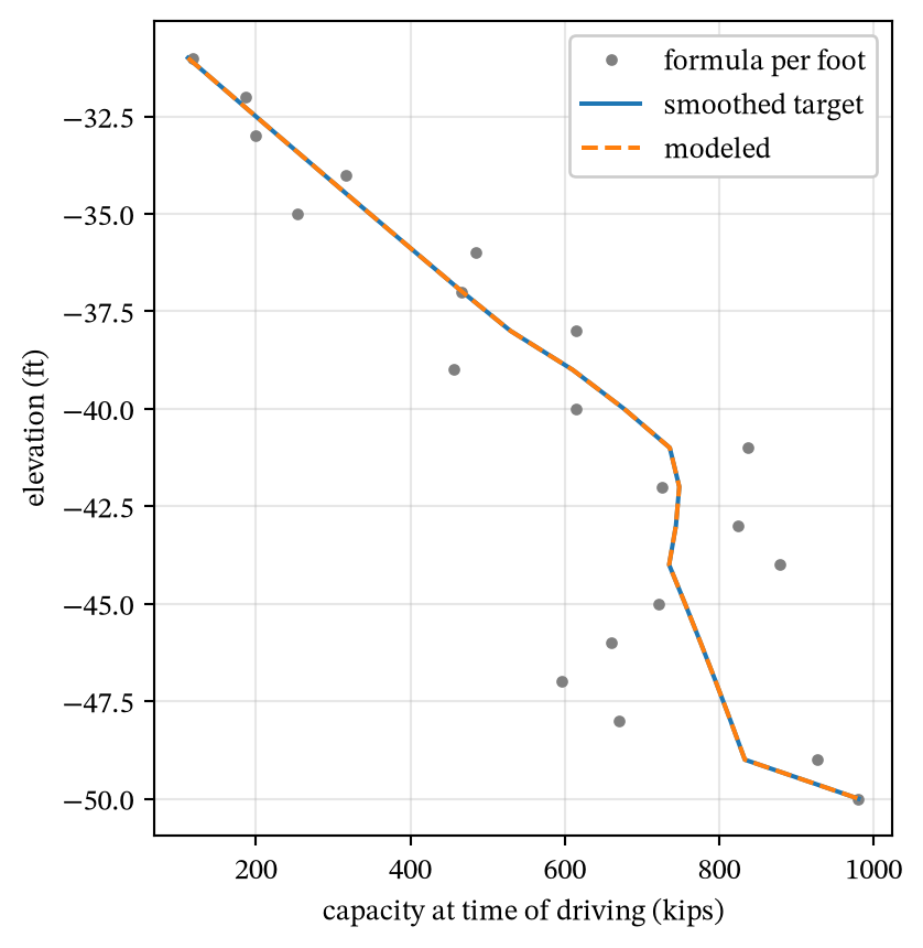

Capacity at the time of driving. The formula capacity of each logged foot (points) is smoothed into the target (solid line), and the analysis reproduces the target with a modeled capacity (dashed line).

Results

The long-term capacity is the shaft resistance after the pore pressure has dissipated plus the toe resistance at the end of the drive.

result.drive.eod_capacity

980.0897207805897

The unit shaft resistance of each foot is lower at the end of the drive than after the excess pore pressure has dissipated. The shaded area between the two curves, multiplied by the pile perimeter, is the setup.

fig, ax = plt.subplots(figsize=(4.5, 5))
ax.plot(drive.fs_eod, drive.elevation, color="C0", label="end of drive")
ax.plot(drive.fs_ltc, drive.elevation, color="C1", label="long term")
ax.fill_betweenx(drive.elevation, drive.fs_eod, drive.fs_ltc, color="C1", alpha=0.25, label="setup")
ax.set_xlabel("unit shaft resistance (ksf)")
ax.set_ylabel("elevation (ft)")
ax.legend(loc="upper right", framealpha=1)
ax.grid(True, alpha=0.3)
plt.show()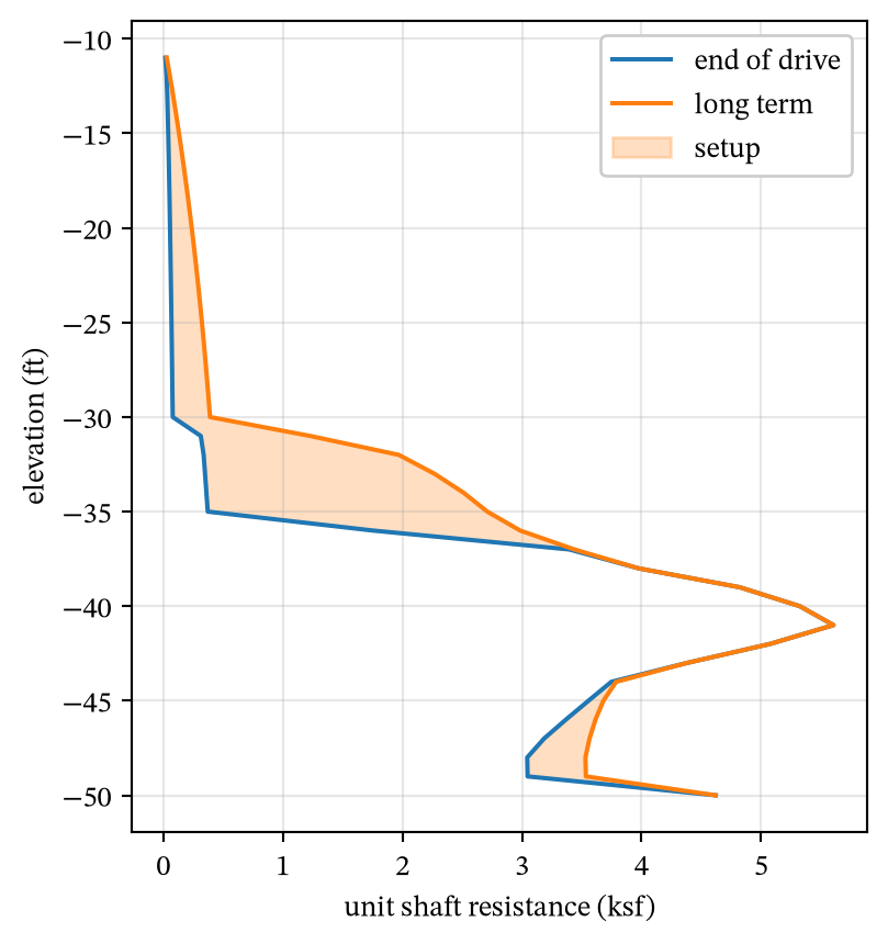

Unit shaft resistance at the end of the drive and after pore-pressure dissipation. The shaded area is the setup.

Summing the unit shaft resistance over the perimeter of each foot, from the mudline down, gives the shaft resistance accumulated above any elevation. The toe resistance is added at the toe, and it is the same in both cases because no toe setup is modeled.

perimeter = drive.pile.perimeter  # ft
shaft_eod = np.nancumsum(drive.fs_eod) * perimeter  # kips, one foot per entry
shaft_ltc = np.nancumsum(drive.fs_ltc) * perimeter

fig, ax = plt.subplots(figsize=(4.5, 5))
ax.plot(shaft_eod, drive.elevation, color="C0", label="shaft, end of drive")
ax.plot(shaft_ltc, drive.elevation, color="C1", label="shaft, long term")
ax.plot(drive.toe_eod, drive.elevation[-1], "o", color="k", label="toe")
ax.set_xlabel("resistance accumulated from the mudline (kips)")
ax.set_ylabel("elevation (ft)")
ax.legend(loc="upper right", framealpha=1)
ax.grid(True, alpha=0.3)
plt.show()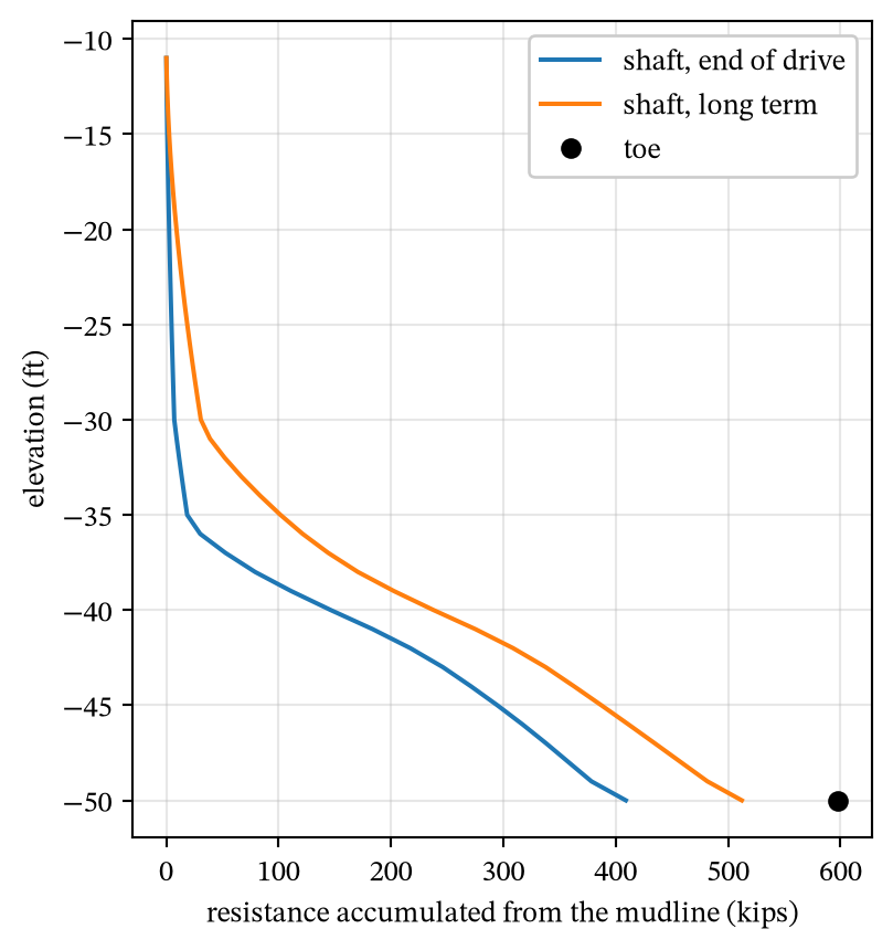

Shaft resistance accumulated from the mudline down, at the end of the drive and in the long term, with the toe resistance at the toe elevation.

toe = drive.toe_eod
rows = [("end of drive", shaft_eod[-1], toe),
        ("long term", shaft_ltc[-1], toe),
        ("setup", shaft_ltc[-1] - shaft_eod[-1], 0.0)]
print(f"{'':14s}{'shaft':>8s}{'toe':>8s}{'total':>8s}   (kips)")
for name, shaft, toe_part in rows:
    print(f"{name:14s}{shaft:8.0f}{toe_part:8.0f}{shaft + toe_part:8.0f}")

                 shaft     toe   total   (kips)
end of drive       409     598    1007
long term          512     598    1110
setup              103       0     103

The walkthrough explains each of these results and the intermediate steps that produce them. The method page and the parameters page document the equations and every option.