This example steps through the method on one of the benchmark piles, pile B-20 of the Pier 4 data set. The one-call analyze builds a capacity target, repeats a sequential characterization pass over a range of friction angles to bound the unlogged top segment, runs the pass once more at the lowest admissible angle, reads the long-term capacity off that result, and optionally repeats the pass again with the uncertainties drawn. Each piece is run here by hand so that its inputs and outputs can be inspected. The method page explains the equations.
Load the record
The log is a CSV with one row per foot: toe elevation, hammer stroke and blows per foot. This inspector recorded the stroke in feet instead of the blow rate, so the stroke column is named; the package converts it to blows per minute on input.
import numpy as np
import matplotlib.pyplot as plt
import driven_pile as dp

pile = dp.Pile.octagonal(width_in=24, length_ft=170.5)
hammer = dp.Hammer(ram_weight=20.0)  # kips

log = dp.DriveLog.from_csv(
    "data/B-20_log.csv",
    pile,
    hammer,
    elevation="elevation_ft",
    stroke="stroke_ft",
    bpf="bpf",
    pile_id="B-20",
)
print(f"{len(log.elevation)} logged feet, "
      f"from {log.elevation.max():.1f} to {log.elevation.min():.1f} ft")
74 logged feet, from -82.4 to -155.4 ft
The fines content comes from a second table of elevation versus percent passing the No. 200 sieve. The mudline at this pile is at elevation -50 ft, 32 ft above the first logged foot.
fines = np.loadtxt("data/B-20_fines.csv", delimiter=",", skiprows=1)
soil = dp.SoilProfile(mudline=-50.0, elevation=fines[:, 0], fines=fines[:, 1])
The capacity target
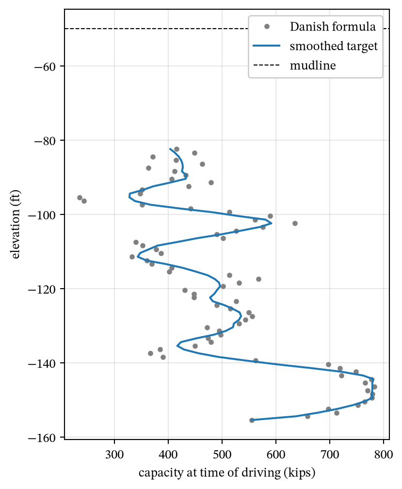
prepare_target applies the recalibrated Danish formula to each foot, smooths the result with a Savitzky-Golay filter, anchors the final foot to its unsmoothed value, and extends the elevation range up to the mudline.
target = dp.prepare_target(log, soil)
print(f"Soil-pile contact: {len(target.elevation)} feet ({target.n_top} unlogged)")
Soil-pile contact: 106 feet (32 unlogged)
fig, ax = plt.subplots(figsize=(4.5, 6))
ax.plot(target.raw_capacity, target.elevation, ".", color="gray", label="Danish formula")
ax.plot(target.capacity, target.elevation, color="C0", label="smoothed target")
ax.axhline(target.mudline, color="k", lw=0.8, ls="--", label="mudline")
ax.set_xlabel("capacity at time of driving (kips)")
ax.set_ylabel("elevation (ft)")
ax.legend(loc="upper right", framealpha=1.0)
ax.grid(True, alpha=0.3)
plt.show()
The characterization pass
Everything after the target is built from one operation, the sequential implicit characterization in run_drive. It takes the target and a friction angle for the unlogged top segment, steps down the pile one logged foot at a time, and returns a per-foot soil profile together with the misfit between the modeled and target capacities. The next three sections repeat it to bound the top segment, inspect one pass foot by foot, and propagate the uncertainties through the model.
The unlogged top segment
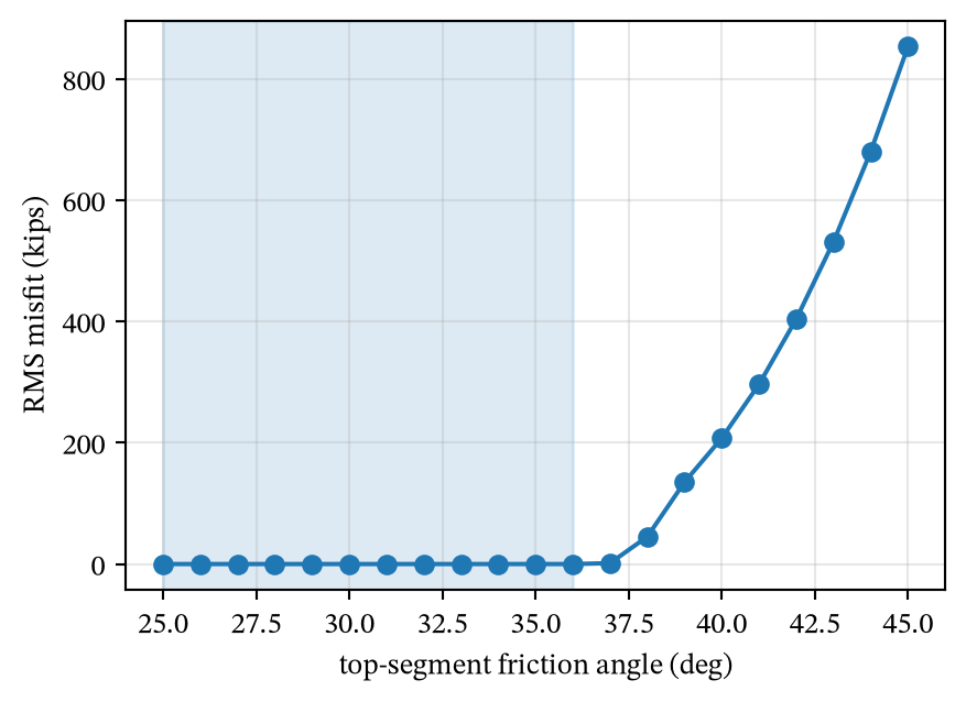
In the example pile pile passed through 32 ft of soil before energy and penetration resistance were recorded. The log says nothing about that soil directly, but the fit below it does, because the shaft resistance of the top segment is subtracted from the target at every logged foot. sweep_top_phi assigns a constant friction angle to the segment, runs one characterization pass for each value from 25 to 45 degrees, and records the root-mean-square misfit of each pass over the logged feet. Each point on the curve below is one full pass.
band = dp.sweep_top_phi(target)
print(f"admissible top-segment friction angle: {band.lo:.0f} to {band.hi:.0f} deg")
admissible top-segment friction angle: 25 to 36 deg
fig, ax = plt.subplots(figsize=(5, 3.5))
ax.plot(band.phi, band.rms, "o-")
ax.axvspan(band.lo, band.hi, color="C0", alpha=0.15)
ax.set_xlabel("top-segment friction angle (deg)")
ax.set_ylabel("RMS misfit (kips)")
ax.grid(True, alpha=0.3)
plt.show()
Within the shaded band, the pass finds equally valid friction angle profiles throughout the log. The deterministic analysis uses the lowest admissible angle for the long-term capacity estimate by default. The probabilistic analysis draws each realization’s angle from the whole band.
Inside one characterization pass
Within a pass, run_drive characterizes each logged foot in sequence from the toe resistance the target demands after subtracting the shaft resistance of the feet above in their current state. At each foot the friction angle and the toe pore-pressure ratio are solved together to self-consistency, since each depends on the other. The blows of that foot also raise the pore pressure of the soil above the toe, so the shaft resistance those feet contribute keeps changing for every later foot in the sequence.
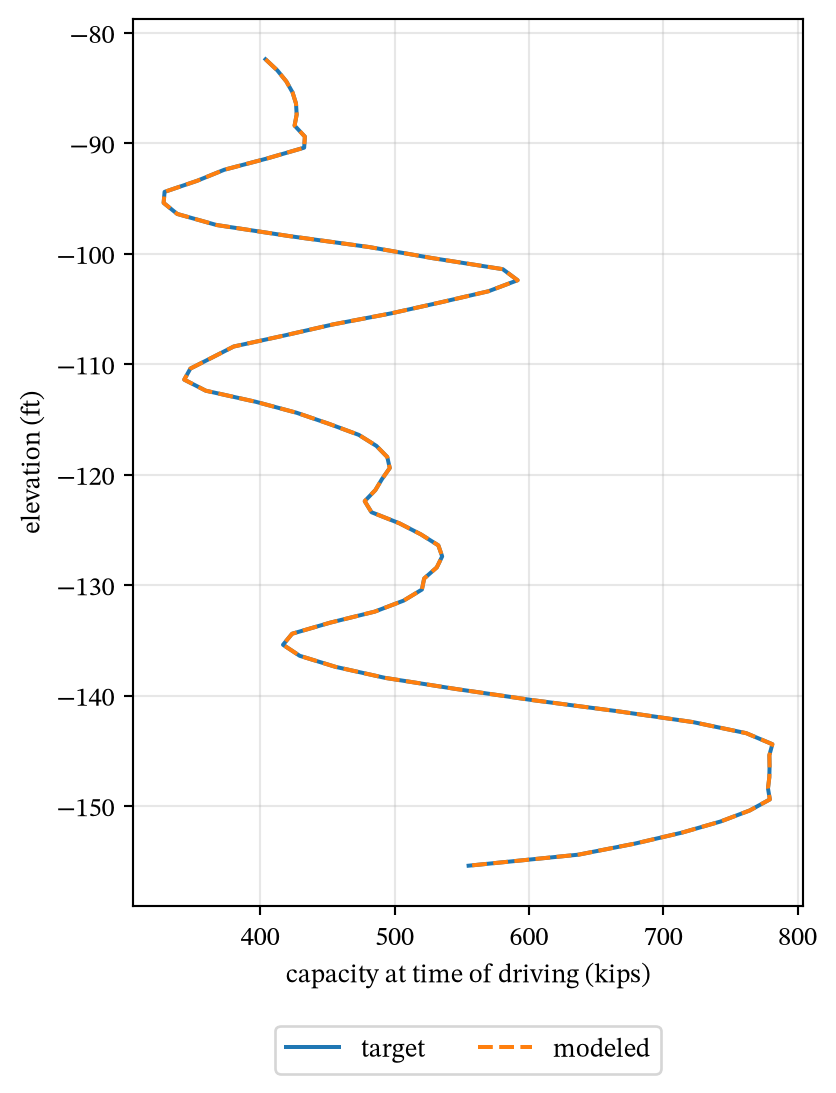
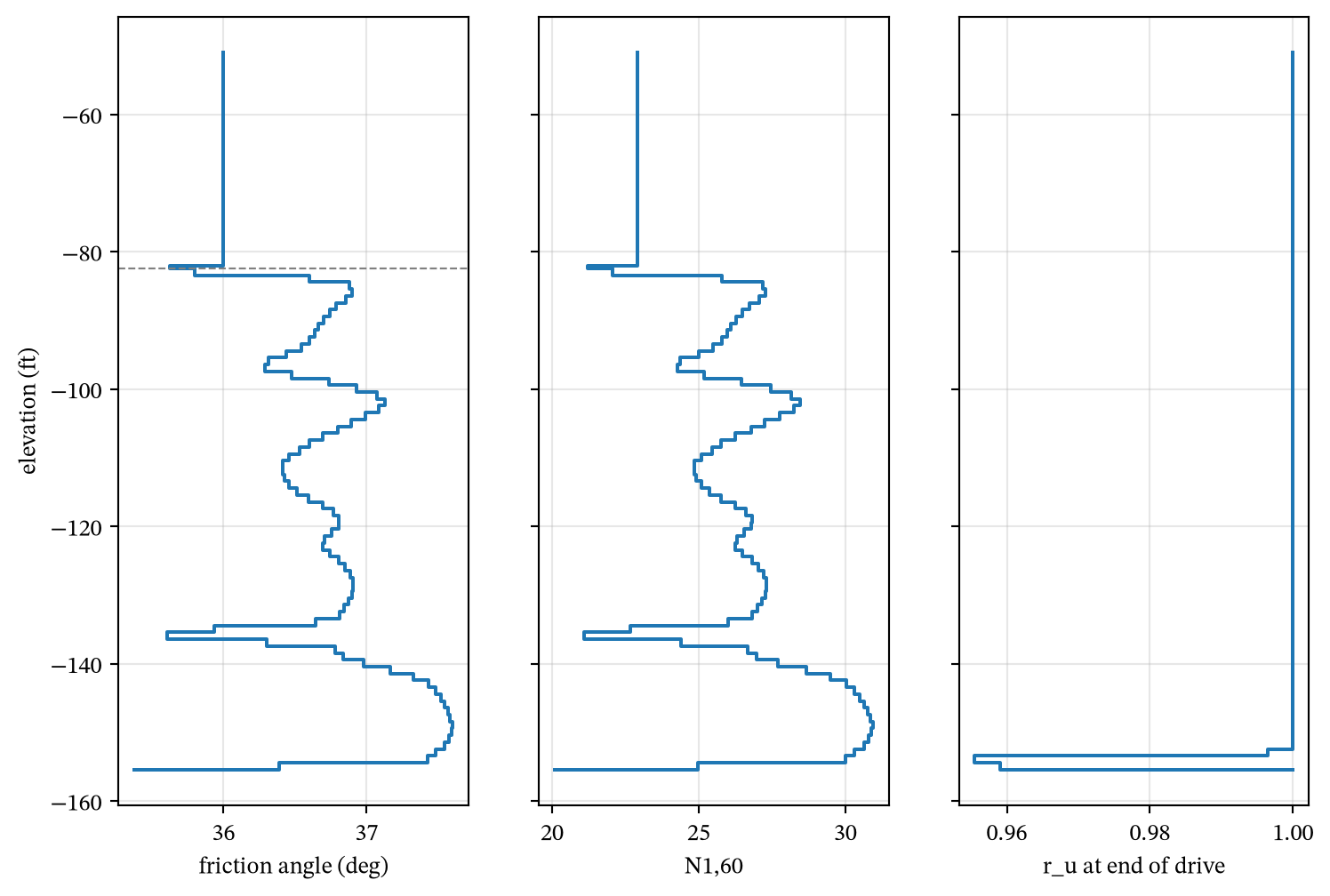
In the result shown below, the characterization pass matches the smoothed target with liquefaction of nearly the entire soil profile.
result = dp.run_drive(target, top_phi=band.hi)
print(f"RMS misfit {result.rms_kips:.1f} kips")
print(f"{100 * result.fraction_liquefied():.0f}% of the logged feet liquefied during the drive")
RMS misfit 0.0 kips
97% of the logged feet liquefied during the drive
result.plot_fit()
plt.show()
result.plot_profile()
plt.show()
Long-term capacity
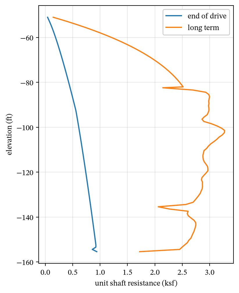
The long-term capacity is the shaft resistance of every foot after its pore pressure has dissipated plus the toe resistance at the end of the drive. long_term_capacity returns the two parts; run_drive has already stored them on the result.
shaft, toe = dp.long_term_capacity(result)
print(f"end of drive  {result.eod_capacity:6.0f} kips")
print(f"long term     {result.ltc:6.0f} kips = shaft {shaft:.0f} + toe {toe:.0f}")
end of drive     555 kips
long term       1877 kips = shaft 1725 + toe 152
fig, ax = plt.subplots(figsize=(4.5, 6))
ax.plot(result.fs_eod, result.elevation, label="end of drive")
ax.plot(result.fs_ltc, result.elevation, label="long term")
ax.set_xlabel("unit shaft resistance (ksf)")
ax.set_ylabel("elevation (ft)")
ax.legend(loc="upper right",framealpha=1)
ax.grid(True, alpha=0.3)
plt.show()
Monte Carlo
monte_carlo repeats the characterization pass once per realization. Each realization draws five uncertain quantities, shown here with their default spreads from MonteCarloOptions:
- Capacity formula bias. One lognormal multiplier on the whole capacity target, mean 1 and coefficient of variation 0.35.
- Scatter of each foot’s capacity. Normal noise added to every logged foot of the target, with the robust standard deviation of the raw formula capacities about the smoothed target.
- Friction angle correlation shift. A uniform shift of up to 2.5 degrees either way in the correlation between friction angle and N_{1,60}, which sets the liquefaction resistance and the residual strength of each characterized foot.
- Cyclic resistance multiplier. One lognormal multiplier on the cyclic resistance ratio, median 1 and logarithmic standard deviation 0.20, which changes the number of blows each foot can take before it liquefies.
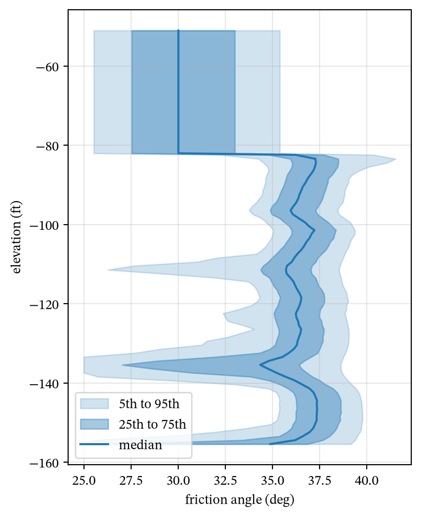
- Top-segment friction angle. Uniform over the admissible band found by the sweep above.
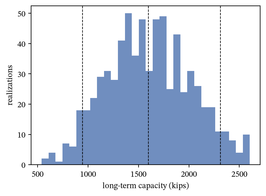
Realizations are added in chunks of 100 until the mean long-term capacity is known to within 2 percent at 95 percent confidence, up to 1200 realizations.
mc_opts = dp.MonteCarloOptions(seed=1)
mc = dp.monte_carlo(log, soil, mc_options=mc_opts, target=target, top_band=band)
mean, half = mc.mean_ci()
q05, q50, q95 = mc.quantiles([0.05, 0.5, 0.95])
print(f"{mc.n} realizations, converged: {mc.converged}")
print(f"mean {mean:.0f} +/- {half:.0f} kips, median {q50:.0f}, 5th to 95th {q05:.0f} to {q95:.0f}")
700 realizations, converged: True
mean 1606 +/- 31 kips, median 1599, 5th to 95th 946 to 2313
fig, ax = plt.subplots(figsize=(4.5, 6))
p = mc.phi_quantiles
ax.fill_betweenx(mc.elevation, p[:, 0], p[:, 4], color="C0", alpha=0.2, label="5th to 95th")
ax.fill_betweenx(mc.elevation, p[:, 1], p[:, 3], color="C0", alpha=0.4, label="25th to 75th")
ax.plot(p[:, 2], mc.elevation, color="C0", label="median")
ax.set_xlabel("friction angle (deg)")
ax.set_ylabel("elevation (ft)")
ax.legend(loc="lower left")
ax.grid(True, alpha=0.3)
plt.show()
Analyze in a single method call
The analyze method performs all of the steps internally and returns the results together. The probabilistic analysis is only performed when requested (by including the optional parameter run_mc=True) The default mode is deterministic.
out = dp.analyze(log, soil) # include run_mc=True for probabilistic result
print(out.drive.ltc == result.ltc, out.top_band.lo == band.lo)